Forecasting H100 spot prices with a Monte Carlo simulation
When there is no forward curve, budgeting future compute expense is impossible. Monte Carlo simulation is one solution to this problem

This analysis is based on proprietary GPU market data collected and curated by Ornn. For more information, visit data.ornnai.com .
Readers have access to the simulation output (Excel) and the simulation engine (Python). See the end of the post.
Introduction
If you’ve ever tried to budget for GPU compute, you know the frustration. Prices fluctuate, sometimes dramatically. Last month’s rate might be 20% higher or lower than today’s. You’re left with an uncomfortable question: should you lock in today’s rate, or wait and hope for prices to drop?
Most of us deal with this uncertainty by picking a number and hoping for the best. We look at today’s price, maybe glance at last week’s, and extrapolate. But this is just guessing with extra steps. There’s a better way, which embraces uncertainty rather than pretending it doesn’t exist. I recently ran a Monte Carlo simulation1 on H100 GPU pricing to explore what the next 90 days might look like. The results were illuminating, not because they predicted the future (they can’t), but because they revealed the shape of uncertainty and what it means for decision-making.
The Uncertainty Problem
Consider the following scenario: you need 1,000 hours of H100 GPU compute over the next three months. The current spot price is $1.70 per hour. Do you buy the capacity now, at today’s price, or wait, in the hopes that the price will drop?
The naive approach is to guess where prices are headed. But guessing is just that, a guess. What if instead of predicting one future, we simulated thousands of possible futures and looked at the distribution of outcomes? That’s the Monte Carlo method in a nutshell. It’s a technique used everywhere from physics to finance to climate modeling. Rather than ask what will the price be?, we ask what’s the range of plausible outcomes, and how likely is each?
Think of it like weather forecasting. A good meteorologist doesn’t say it will rain tomorrow. They say there’s a 70% chance of rain. Monte Carlo gives us that same probabilistic framing for price forecasts. We lose the comfort of false certainty, but we gain an honest picture of what we’re actually facing.
A Brief Detour: Why GPU Prices Aren’t Like Stocks
Before diving into the results, it’s worth understanding one key assumption behind the simulation. Stock prices, in theory, can rise indefinitely. There’s no fundamental ceiling. Amazon was once $1.50 a share; now it’s over $200.
GPU compute pricing behaves differently. It’s more like a commodity. When prices spike, cloud providers have an incentive to add capacity, and customers defer non-urgent workloads. When prices crash, the opposite happens. Over time, prices tend to oscillate around some equilibrium level rather than trending off to infinity.
The simulation uses a model designed for this rubber band-like behavior. Prices get pulled back toward a long-term average. If current prices are below that average (as they are now), the model expects them to drift upward. If they’re above, it expects them to fall. The further prices deviate from the mean, the stronger the pullback.
This is a simplification, of course. Reality is messier. But it’s a reasonable starting point for thinking about commodity-like markets.
What I Fed Into the Model
The simulation drew on 90 days of real H100 spot pricing data from the Ornn’s data, covering late October 2025 through late January 2026. During this period, prices peaked around $2.21 in mid-November before declining about 22% to the current $1.70.
From this history, the model estimated three key parameters:
Long-term mean price: $1.88/hour (the historical average)
Volatility: about 51% annualized (prices can swing meaningfully)
Mean reversion speed: relatively fast (prices don’t stay far from the mean from long).
With these parameters in hand, I simulated 5,000 possible price paths over the next 90 days. For each path, I calculated what it would cost to consume 1,000 GPU hours spread evenly across the period.
The result: 5,000 different cost outcomes, each representing one plausible future.
What the Simulation Reveals
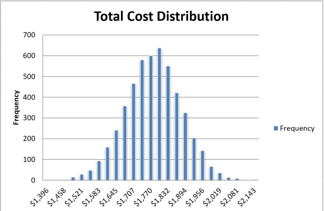
The distribution of costs looked like a bell curve centered around $1,7952. Here are the key numbers:
Central estimates:
Mean cost: $1,795
Median cost: $1,796
The range of outcomes:
5th percentile (lucky scenario): $1,629
95th percentile (unlucky scenario): $1,960
Absolute minimum across all simulations: $1,396
Absolute maximum: $2,174
The strategic question: buy now or wait?
Buying 1,000 hours today at spot: $1,700
Probability of beating that by waiting: just 16.6%
The last number is the key insight. If you lock in today’s rate, you’re getting a better deal than roughly 5 out of 6 simulated futures. The current price of $1.70 is about 10% below the historical average, and the model expects prices to drift back up toward that average over time.
To put it another way: waiting is a bet against the base case. It might pay off. Approximately 1 in 6 times, you’d come out ahead, but you’re swimming against the current. The model sees today’s low prices as an anomaly that will likely correct.
Visualizing Uncertainty
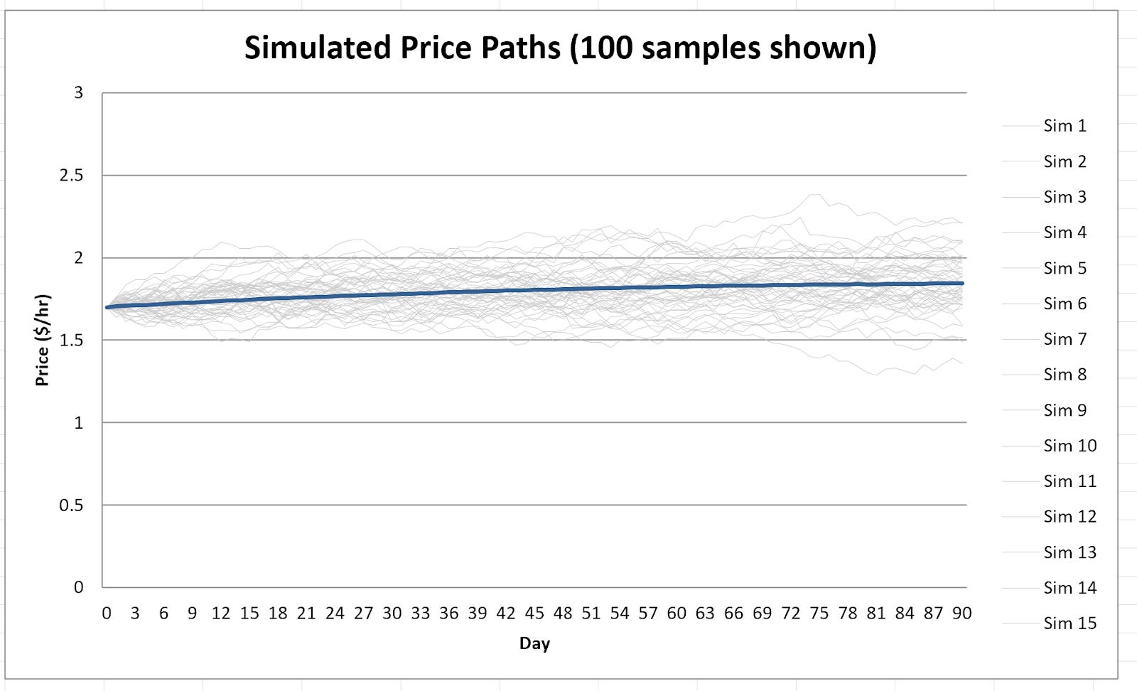
Numbers only tell part of the story. Looking at the simulated price paths makes the uncertainty tangible.
All 5,000 paths start at the same point: $1.70 on day zero. But they immediately begin to diverge. Some drift higher, some lower. A few shoot up toward $2.20; a few sink below $1.40. By day 90, the paths span a range of about 50 cents, from roughly $1.58 at the 5th percentile to $2.11 at the 95th.
The fan-shaped spread of paths illustrates a fundamental truth: uncertainty compounds over time. We have a decent sense of where prices might be tomorrow, but 90 days out, the range of possibilities is wide.
The cost distribution, which measures what you’d actually pay for your 1,000 hours, inherits this uncertainty. It’s a bell curve with most common outcomes clustered between $1,700 and $1,900, but with tails extending in both directions.
What This Means for Decision-Making
So what should you actually do with this information?
If you need GPU compute and can lock in today’s rate, the simulation suggests that’s probably a good deal. You’re buying below the expected future average. Waiting could save you money. There’s about a 1-in-6 chance of that. But the odds favor locking in.
If you have flexibility on timing, you might watch for prices to dip further before committing. The simulation shows some paths where prices fall into the $1.50s. But be aware that you’re betting against the base case.
For budgeting purposes, the 90% confidence interval ($1,629 to $1,960) gives you reasonable planning bounds. If you’re conservative, budget for the 95th percentile. If you’re optimistic, use the median. Either way, you’re making an informed choice rather than a blind guess.
If you can shift your usage pattern, there might be additional savings available. The simulation assumes uniform consumption across all 90 days. But if you could front-load your usage, meaning you consume more hours now while prices are low, you’d likely do better than the expected case. Conversely, back-loading (more usage later) increases your exposure to potential price increases. The model doesn’t capture this flexibility, but it’s worth considering in practice.
The Limitations of This Model
I’d be doing you a disservice if I presented this analysis without caveats. Monte Carlo simulation is a powerful tool, but it’s not magic. Here’s what it can’t do:
It can’t predict structural changes. The model assumes prices will continue behaving the way they have historically. If the market fundamentally shifts–say a flood of new GPU supply comes online, or a major new AI model spikes demand–the historical patterns won’t hold. The long-term mean of $1.88 is really just the average of the last 90 days. It’s not a law of nature.
It doesn’t capture sudden shocks. The simulation generates smooth, continuous price paths. Real markets can jump discontinuously. Think about a supply disruption, a policy change, or a surprise product announcement. These black swan events aren’t in the model. The simulation’s well-behaved bell curve may understate the probability of extreme outcomes in either direction.
The parameters themselves are uncertain. The volatility estimate, the mean reversion speed: these are derived from limited data and carry their own error bars. The simulation treats them as known constants, which overstates our confidence. In reality, even the inputs to the model are uncertain.
90 days of history is thin. Ideally, you’d calibrate a model like this on years of data, not months. With only 90 observations, the parameter estimates are noisy. A different 90-day window might yield different results. The calibration period happened to include a peak-to-trough cycle. Had it captured a different pattern, the model’s expectations would shift.
It assumes you can always buy at spot. The model presumes you can purchase GPU hours whenever you want at the prevailing market price. In practice, capacity constraints or reservation requirements might force you to pay premiums during high-demand periods.
None of this invalidates the exercise. It just means you should treat the outputs as one input among many, not gospel truth. The simulation is a thinking tool, not a crystal ball.
The Bigger Picture: Thinking in Probabilities
Beyond the specific question of GPU pricing, there’s a broader lesson here about decision-making under uncertainty.
Most business planning uses single-point forecasts. “We’ll need $50,000 for compute next quarter.” But this false precision obscures the uncertainty that actually exists. What’s the range? How confident are we? What are the tail risks?
Monte Carlo simulation forces you to confront these questions. Instead of one number, you get a distribution. Instead of certainty, you get probabilities. This is uncomfortable at first, but it’s more honest.
The tools for this kind of analysis are increasingly accessible. APIs like Ornn provide real-time market data. Python libraries handle the mathematical heavy lifting. You don’t need a PhD in quantitative finance to run these simulations. The barrier isn’t technical; it’s conceptual. It’s learning to ask “what’s the distribution of outcomes?” instead of “what’s the answer?”
A Market Matures
There’s one more thing worth noting. The fact that we can even do this analysis–treat GPU compute like a commodity with price indices, volatility metrics, and mean-reverting dynamics–reflects how much this market has matured.
A few years ago, GPU pricing was opaque and fragmented. You’d check a few cloud providers, maybe ask around on Twitter, and piece together a rough sense of rates. Today, we have indices tracking spot prices across providers, APIs serving historical data, and enough market depth to make statistical modeling meaningful. GPU compute is becoming a tradable commodity, and with that comes the analytical toolkit we use for other commodities.
For those of us who consume compute, that’s good news. More transparency means better decisions. More data means we can move beyond gut feelings to quantified uncertainty. The volatility doesn’t go away, but at least we can see its shape.
And perhaps that’s the real takeaway from this exercise. Uncertainty is unavoidable. But uncertainty you can measure and reason about is far better than uncertainty you pretend doesn’t exist. A probability distribution won’t tell you what will happen, but it will tell you what you’re betting on, and what the odds are.
That’s worth knowing, whether you’re budgeting for GPU hours or making any decision where the future is unclear. Which, of course, is most decisions worth making.
If you enjoy this newsletter, consider sharing it with a colleague.
I’m always happy to receive comments, questions, and pushback. If you want to connect with me directly, you can:
follow me on Twitter,
connect with me on LinkedIn, or
send an email to dave [at] davefriedman dot co. (Not .com!)
The simulation engine was built by Claude Opus 4.5.
Readers can download the simulation engine (Python) and output (Excel) here. That’s a Google Drive link; if your organization blocks Google Drive, send me an email (dave at davefriedman dot co (not .com)) indicating that you are a paid subscriber, and I will provide you with the files. You will need an API key for Ornn’s data if you want to run the script and retrieve data. Ornn’s web site is here.
Monte Carlo doesn't really let you forecast. It offers a range of outcomes, and potentially correlated effects. It's a risk assessment.