GPU Obsolescence is Complicated

There are three obsolescence curves, not one.

At Nvidia’s GTC conference in March 2025, Jensen Huang delivered one of his trademark lines about the company’s previous-generation Hopper chips: “In a reasoning model, Blackwell is 40 times the performance of Hopper. Straight up. Pretty amazing. I said before that when Blackwell starts shipping in volume, you couldn’t give Hoppers away.”

Later in 2025, CoreWeave’s Michael Intrator told CNBC that a batch of H100s had come off contract and been immediately rebooked at 95% of their original price. Bernstein analyst Stacy Ragson noted that even five-year-old A100 chips were generating comfortable margins, with capacity at GPU cloud providers nearly fully booked.

Same chip. Same moment in time. Two completely contradictory claims about its value.

The resolution isn’t that one of them is lying. It’s that they’re talking about different markets for the same physical asset, and the industry doesn’t have a framework for that. Jensen is talking about frontier training. Intrator is talking about inference. They’re both right, and they’re both incomplete, because they’re each describing one slice of a more complex picture that nobody has bothered to articulate clearly.

The Single-Curve Fallacy

The GPU depreciation debate is one of the loudest arguments in AI finance, and its framing is almost entirely wrong.

On one side: Michael Burry, the Big Short guy, arguing that hyperscalers are overstating the useful life of their AI chips, and understating depreciation. He pegs actual useful life at two to three years and says companies are inflating earnings as a result. Jim Chanos and Aswath Damodaran have made similar arguments. Jonathan Ross, the Groq founder, now at Nvidia after the $20 billion licensing deal, argued for one-year amortization schedules. Princeton’s Center for Information Technology Policy published a piece framing the core issue as chips having “a useful lifespan of one to three years due to rapid technological obsolescence and physical wear.”

On the other side: hyperscalers booking five- to six-year depreciation schedules, CoreWeave doing the same, and analysts like SiliconANGLE’s research team arguing that today’s training infrastructure will support future workloads, extending useful life well beyond the initial purpose. They point to the value cascade: chips waterfalling from training to inference to general-purpose compute as newer generations take over the top slot.

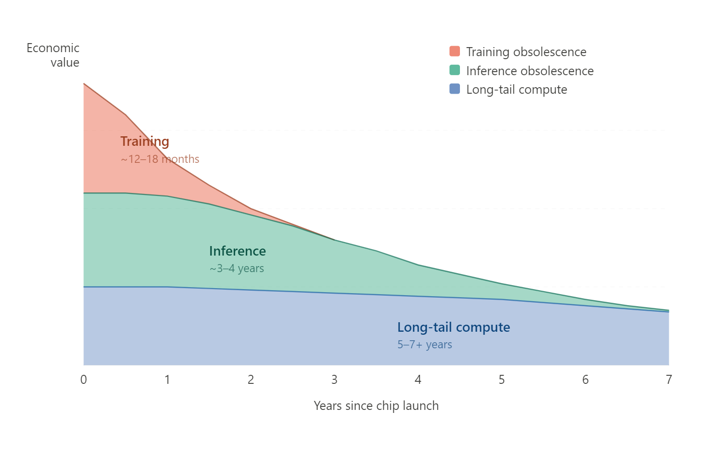
Every one of these participants is implicitly assuming that a GPU has a single obsolescence curve: one line on a chart, declining from “new and valuable” to “expensive paperweight.” The entire debate is about the slope of that line. But a GPU doesn’t have one obsolescence curve. It has several, and they are stacked on top of one another, each with a different shape, a different slope, and different underlying drivers. The useful life of a chip is not a single number. It’s a composite: the sum of the economic value generated across multiple workload tiers over time.

Three Curves, One Chip

Graph created with Claude Opus 4.6. The total economic value at any given point is the sum of all three layers. The rapid collapse of the training slice doesn’t mean the chip has lost all its value. It just means that the highest-value use case has migrated to newer silicon.

Curve 1: Training Obsolescence

This is the steep one. This is the one everyone sees, because it’s the most dramatic.

A chip becomes training-obsolete when the next generation makes it uneconomical to start a new large-scale training run on old hardware. The driver is raw FLOPS-per-dollar at the frontier. If Blackwell delivers 4x the training throughput of Hopper at comparable total cost of ownership, then no rational actor is going to start a new frontier training run on Hoppers. The economics of a three-month, mult-hundred-million-dollar training run are brutally sensitive to compute efficiency. You can’t make up a 2x gap by renting cheaper old chips. The opportunity cost of time dominates everything.

The clock on this curve is basically Nvidia’s release cadence: 12 to 18 months. When Jensen says “you couldn’t give Hoppers away,” he’s describing the training obsolescence curve. And for training, he’s right. Once Blackwell is available at scale, Hoppers are functionally worthless for new frontier training jobs.

This is the curve Burry is pricing. This is the curve the Princeton piece is describing. And if you think this is the only curve, you get a useful life of 1-3 years and you conclude the hyperscalers are cooking the books.

Curve 2: Inference Obsolescence

This curve is much shallower, and the drivers are fundamentally different.

A chip becomes inference-obsolete not when a better chip exists, but when the blended cost of migrating to that better chip is less than the cumulative savings from lower cost-per-token on the new hardware. That’s a much higher bar than the training case, for several reasons.

First, inference is throughput-per-dollar, not peak-FLOPS. The performance delta between generations matters less in inference than in training, because you’re optimizing for cost per unit of output, not time to completion. An H100 doing inference on a model that was trained on H100s is perfectly adequate hardware. It doesn’t need to be the fastest thing in the building. It needs to be cheap enough per token to be profitable.

Second, inference workloads have enormous switching costs that training workloads don’t. Software stacks are mature and deeply integrated. Engineers know the chip’s quirks. Quantization and optimization work has already been done for the specific hardware. CoreWeave’s management made exactly this point: demand for H100s remains strong because the software libraries are mature and engineers are deeply familiar with them.

Third, inference demand is growing so fast that older chips don’t get displaced. They get pushed down the demand stack. There is so much inference work to be done that even if Blackwell is better per-token, there’s more than enough token demand to keep Hoppers busy. Older chips don’t become unemployed; they just take a pay cut.

The result: a chip that’s training-obsolete in 18 months might be inference-competitive for 3-4 years. The CoreWeave rebooking data–H100s at 95% of original contract price–is a direct market signal of this curve’s shape. So is the fact that A100 capacity at GPU cloud providers is, per Bernstein, nearly fully booked.

Curve 3: Long-Tail Compute

This one is nearly flat.

Below the frontier training and high-volume inference tiers, there’s a massive pool of workloads that use GPUs but don’t need anything close to the latest generation: ad optimization, recommendation engines, classical ML, fine-tuning smaller models, video transcoding, scientific simulation, non-AI accelerated compute. V100s are still running these jobs. T4s are everywhere. An A100 in 2029 will still be dramatically faster than any CPU for parallelizable numerical work.

The obsolescence trigger for this tier isn’t a new chip. It’s one of two things: physical failure (the chip dies) or a power-cost crossover point where the electricity required to run the old chip exceeds the cost of replacing it with something newer and more power-efficient. Both of these are measured in years, not quarters.

One MBI Deep Dive piece captured this dynamic: a hyperscaler like Google, Amazon or Microsoft runs everything from cloud databases and video transcoding to scientific simulations and internal analytics. For them, a three-year-old H100 may not be obsolete, but can be redeployed to accelerate countless other tasks, delivering significant performance uplift over traditional CPUs and generating economic value for years.

This is the curve the hyperscalers are implicitly pointing to when they defend six-year depreciation schedules. But they’re not articulating it as a separate curve with its own dynamics. They’re blending it into a single value cascade narrative that muddles the whole picture.

Why No One Thinks This Way

If the multi-curve framework is more accurate, why hasn’t anyone articulated it?

A few reasons.

The accounting frame can’t express it. GAAP demands one useful life estimate per asset class. The entire Burry-vs-hyperscaler debate is organized around a single parameter: should it be two years or six? Once you’re arguing about one number, you’ve implicitly accepted one curve. Component depreciation under ASC 360 lets you separate the GPU module from the chassis and networking, but even that’s a physical decomposition, not a workload decomposition. There is no accounting standard that says “depreciate this chip on three different schedules depending on what it’s doing.” The framework literally cannot accommodate the reality.

The incentives favor simplicity. Jensen wants one curve because it sells Blackwell. Burry wants one curve because it supports his short thesis. The hyperscalers want multiple curves because they protect their earnings. A multi-curve framework is inconvenient because it introduces ambiguity. It says: you’re all partially right, and the actual answer depends on demand composition by workload tier over time. That’s not a trade. It’s not a headline. It’s not an earnings defense. It’s a shrug accompanied by a complicated chart.

The knowledge gap is severe. To decompose obsolescence into workload-specific curves, you need to understand the compute demand taxonomy in detail. You need to know that inference has different performance requirements than training, that classical ML optimization is even less demanding, that fine-tuning sits somewhere in between. Most of the people opining on GPU depreciation can’t tell you what a T4 is being used for right now or why a V100 still has economic value. They know “Nvidia makes chips, new chips are faster, old chips lose value.” You can’t build a multi-curve model if you don’t even know what the curves are.

The people who do think this way aren’t publishing. The firms that actually model recovery waterfalls–Magnetar, Castlake, the structured credit shops underwriting GPU-backed facilities–are the ones with the mental model closest to what I’m describing. In structured finance, you always ask: if the top tranche of demand disappears, what’s the next-best use and what does it pay? That’s the workload-cascade question, decomposed by tier. These firms are almost certainly modeling multiple recovery scenarios by workload tier. But they’re not writing blog posts about it. They’re writing term sheets.

Why This Matters

If you’re an equity analyst modeling hyperscaler depreciation, the single-curve framework leads you to one of two bad answers: either you accept the six-year schedule and miss the risk that training-tier demand for current-gen chips erodes in 18 months, or you accept Burry’s two-year estimate and miss the value embedded in inference and long-tail demand. The multi-curve framework gives you a more honest answer: the first two years of depreciation should be steeper (capturing the rapid loss of training-tier value), and the back four years should be shallower (capturing the persistent inference and long-tail demand). That’s an accelerated depreciation schedule, but it’s not the cliff that the bears imagine.

If you’re a lender underwriting GPU-backed facilities, the stacked-curve model gives you a collateral recovery waterfall. If training demand for this chip disappears tomorrow, what’s the inference demand floor? If inference demand erodes over time, what’s the long-tail floor? What does each tier pay? How deep is the demand pool at each level? This is how structured credit people already think about commercial real estate, aircraft, and shipping. The same mental model applies here. The residual value of a GPU isn’t “what’s this chip worth in three years?” It’s “what’s the lowest-value workload this chip can still economically serve, and how much demand exists at that tier?”

If you’re a policymaker thinking about AI infrastructure investment, the multi-curve model reframes the risk. The bearish narrative–hundreds of billions in chips becoming e-waste in two years–is overstated, because it’s pricing only the training curve. But the bullish narrative–chips retain value for six years, everything’s fine–is also overstated, because the highest-value use case does erode fast, even if the asset retains some economic utility. The truth is a portfolio of decaying optionalities, and the aggregate value depends on the depth and persistence of demand at each tier.

The Uncertainty Underneath

I want to be clear: getting the framework right doesn’t make the problem easy. Each of the three curves has enormous uncertainty.

The training curve depends on Nvidia’s execution on future architectures, on whether alternative silicon (AMD, custom ASICs, Trainium) fragments the frontier training market, and on whether training run sizes continue scaling or plateau.

The inference curve depends on model architecture evolution (will future models be more or less hardware-agnostic?), quantization and distillation techniques (which extend the useful life of older chips by letting them run lighter versions of newer models), and the overall growth rate of inference demand (which determines whether older chips get displaced or merely pushed down-market).

The long-tail curve depends on power costs, on whether cloud providers continue offering older GPU instances or retire them in favor of denser new hardware, and on how quickly non-AI accelerated workloads grow.

None of this is easy to forecast. But at least the multi-curve framework makes you wrong for the right reasons: because you misjudged a specific variable in a correctly-structured model, not because you were solving the wrong equation entirely.

The Bottom Line

The GPU depreciation debate is a 2-years-vs-6-years argument, and both sides are answering the wrong question. A GPU does not have a useful life. It has several useful lives, stacked on top of each other, each serving a different market with different performance requirements, different switching costs, and different demand dynamics.

Training obsolescence is fast. Inference obsolescence is slow. Long-tail compute obsolescence is glacial. The aggregate economic life of a chip is the sum of all three, and it looks nothing like any single curve that anyone in this debate is drawing.

---

If you enjoy this newsletter, consider sharing it with a colleague.

I’m always happy to receive comments, questions, and pushback. If you want to connect with me directly, you can:

• follow me on Twitter,

• connect with me on LinkedIn, or

• send an email to dave [at] davefriedman dot co. (Not .com!)